Network Switches are the evolution of Hubs and Repeaters, and enable the creation of networks by connecting multiple devices together. They are critical components in computer networking and are used to connect devices like computers, printers, and servers in local area networks (LANs) and wide area networks (WANs). Switches are designed to manage the flow of data between devices, ensuring that each device is able to communicate efficiently and effectively with other devices on the network.

Switches (Layer-2 Switching) do not receive and transmit data throughout every port, like hubs, but instead examine a packet's destination by checking the MAC address. The destination MAC address is always located at the beginning of the packet (see Ethernet II Protocol article) as shown below:

A switch will then forward the frame via the intended port, or out all its ports, depending if it finds an entry for this MAC address in its memory (filter table). This process is explained in more detail later in this article.

Switches use Application Specific Integrated Circuits (ASIC's) to build and maintain filter tables. Layer-2 switches switch packets between ports at a faster rate compared to routers, simply because routers need to examine the Network layer (layer-3) information of the packet, which is higher up in the OSI model and requires additional processing power and time.

• They provide hardware based bridging (MAC addresses)
• They work at wire speed, therefor have low latency
• They come in 3 different types: Store & Forward, Cut-Through and Fragment Free (Analysed later)

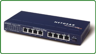
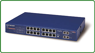
Physically, it's difficult to tell a switch from a hub as they both look alike. The difference between them is under the hood! The photos below show a 8-port hub (left) and 18 port switch (right). Notice the switch provides two ports on the far right - these are uplink ports, allowing the switch to connect to the rest of the network (other switches):

The Three Operating Stages of a Network Switch

Network switches operate in three stages: learning, forwarding, and filtering.

• Stage 1: Learning
  
• Stage 2: Forwarding
• Stage 3: Filtering
• Loop Avoidance (Optional)
  

Overall, the three stages of learning, forwarding, and filtering allow the network switch to effectively manage the flow of data on a computer network, ensuring that devices can communicate with each other efficiently and securely.

Stage 1: Address Learning

The diagrams below shows how frames are forwarded out all switchports when the destination MAC address is unknown (there is no entry in the MAC address table). This is usually the case when a switch is initially powered on (or has an empty MAC address table). In this example, Node 1 sends a packet desitined to Node 2. The switch at this point has already inserted Node1's MAC address in its MAC address table:

And after the first frame has been successfully received by Node 2, it then sends a reply to Node 1. The switch is now aware of the two nodes MAC addresses and will send all frames between them, out through the switchports they are connected to:

Notice how Node 2's frame destined to Node 1, is not transmitted out every switchport . The switch is now aware of the switch ports both Node 1 and Node 2 are connected to:

Forward/Filter Decision

When a frame arrives at a switch, the switch examines the destination MAC address of the frame to determine which port it should forward the frame to. As noted previously, the switch maintains a table, called the MAC address table or the CAM table, which maps MAC addresses to their associated switch ports. If the destination MAC address is already in the MAC address table, the switch will forward the frame out the corresponding port. If the destination MAC address is not in the table, the switch will flood the frame to all ports except the one on which it was received.

This is known as unknown unicast flooding and ensures that the frame reaches its intended destination. Once the frame reaches its destination, the switch updates its MAC address table with the source MAC address and the port on which the frame was received, so that it can forward future frames to that device more efficiently.

Loop Avoidance (Optional) - Spanning-tree protocol

The Spanning Tree Protocol (STP) is a networking protocol designed to prevent loops in networks with redundant links. When multiple paths are available between devices in a network, a loop can occur if the same packet is forwarded indefinitely between devices. This can cause network congestion and ultimately result in a network outage. STP solves this problem by creating a loop-free logical topology for the network.

STP works by selecting a root bridge, which is the device that has the highest priority in the network. Once the root bridge and port roles have been determined, STP builds a tree-like topology that includes all devices in the network. The topology is designed to ensure that there is only one active path between any two devices, which prevents loops from occurring. The tree-like topology is also designed to provide redundancy in the event of a link failure. If a link fails, STP recalculates the topology to find a new path between the affected devices.

STP has several variations, including Rapid Spanning Tree Protocol (RSTP) and Multiple Spanning Tree Protocol (MSTP). RSTP is an improvement on STP that reduces the time it takes for the network to recover from link failures. MSTP is a protocol that allows multiple VLANs to be mapped to a single spanning tree instance, which reduces the number of spanning tree instances required in a network.

In summary, STP is a networking protocol that creates a loop-free logical topology for networks with redundant links. By selecting a root bridge and assigning roles to other devices in the network, STP ensures that there is only one active path between any two devices, which prevents network congestion and outages. STP operates in three phases and has several variations, including RSTP and MSTP.

Switching Modes: Store-and-forward, Cut-through & Fragment-free

There are three primary switching methods: store-and-forward, cut-through, and fragment-free. While all three methods are analyzed in detail, the below diagram shows the portion of a receiving frame a switch will process (check), before forwarding it out its intended port(s):

Store-and-forward switching is the most common method and involves the switch receiving and buffering the entire frame before forwarding it to the destination device. During this process, the switch performs error checking on the frame to ensure it is complete and error-free. If the frame is damaged, the switch discards it. Store-and-forward switching is considered the most reliable switching method as it ensures that only complete, error-free frames are forwarded, but it also has the highest latency due to the buffering and error checking process.

Cut-through switching is a faster method than store-and-forward, as the switch starts forwarding the frame as soon as it reads the destination MAC address. With cut-through, the switch only buffers the minimum amount of the frame (up to the destination MAC address section) required to determine the destination port. Cut-through switching is faster than store-and-forward because it does not wait for the entire frame to be received and verified before forwarding. Keep in mind that this method can forward corrupted frames since there is no error checking before forwarding.

Fragment-free switching is a variation of cut-through switching that reads the first 64 bytes of a frame before forwarding it. This is done to prevent forwarding of frames that may have been damaged during transmission. In general, the first 64 bytes of a frame contain the frame header, which includes the source and destination MAC addresses, as well as the frame type. By reading the first 64 bytes, fragment-free switching can ensure that the frame is not corrupted without having to wait for the entire frame to be received.

Generally speaking, store-and-forward switching is the most reliable but has the highest latency due to the buffering and error checking process. Cut-through switching is faster than store-and-forward but can forward corrupted frames. Fragment-free switching is a variation of cut-through that reads the first 64 bytes of a frame before forwarding it, which reduces the likelihood of forwarding corrupted frames. The choice of switching method depends on the specific needs of the network, and a combination of these methods can be used in larger networks to achieve a balance between reliability and speed.

Network Switches Memory Buffer

The memory buffer in a network switch is an essential component that plays a critical role in ensuring efficient and reliable data transmission. The buffer is responsible for temporarily storing incoming data packets before forwarding them to their destination. Without a memory buffer, the switch would be unable to handle high volumes of network traffic, resulting in packet loss and network congestion. The buffer also helps to prevent data loss by holding packets in case of congestion, allowing time for the switch to clear the congestion and forward the packets. The size of the buffer is an important factor in determining the performance of the switch, as it determines the amount of data that can be temporarily stored. A switch with a larger buffer can handle more traffic and is better equipped to handle bursts of data. As such, the memory buffer is a critical component in ensuring reliable and efficient network performance.

• Bridges are software based, while switches are hardware based because they use an ASICs chip to help them make filtering decisions.

• Bridges can only have one spanning-tree instance per bridge, while switches can have many.

• Bridges can only have upto 16 ports, while a switch can have hundreds!

Summary

This article explained how network switches operate and compared them with hubs. We examined the three operating stages of a switch: learning, forwarding, and filtering, and provided an overview of network loop avoidance with the help of the Spanning-Tree protocol. We talked about the three switching modes used by switches to forward frames: Store-and-forward, Cut-through & Fragment-free, and how the switch memory buffer plays a critical role in this process. Lastly touched on network bridges and how they we used in the early days to segment networks.

One of the most used terms in network is LAN (Local Area Network). It’s a form of network that we encounter in our daily lives, at home, at work, study, and in various other areas of life. Unless working specially in the field of Wide Area Networks (WAN), you will come across a LAN pretty much everyday. A key protocol used to maintain efficiency within a LAN is the Spanning Tree Protocol (STP), which is standardized as IEEE 802.1D.

Without this protocol our LANs would rapidly become congested, with frames looping throughout the network infinitely, making network devices unstable. This protocol is implemented on switches, as switches deal with network data at the frame level. But before going ahead with a full blown explanation of what STP is, it is important to understand the ‘problem’ that STP prevents and how it improves a LAN’s performance. Let’s go through some salient features of a LAN first.

One of the most important devices within a LAN is a network switch. All standard switches are Layer 2 devices i.e. they work at the level of frames. A frame is the unit of transmission in a link layer protocol and consists of a link-layer header followed by a packet. Without going into too much detail, a switch communicates in terms of frames. Users interested learning more about frames, can visit our Ethernet Frame Formats section where they'll find plenty of useful information and 3D representations of the various Ethernet frames. Apart from the higher layer data encapsulated by the frame, it carries two other important pieces of information, the Source MAC Address and the Destination MAC Address. It’s important to make a note of this as it becomes vital in our understanding of how a switch works and for STP itself.

How Does A Switch Work?

It must be noted that, before starting on this tutorial, it is best to have an understanding of how a switch works. If not then all is not lost. Users can always look up existing switch principles covered under the Switches & Bridges article.

Understanding of the following topics is essential for STP:

• How a switch finds MAC Addresses of new hosts
• How a switch populates its MAC Address tables
• How a switch deals with an incoming frame when it doesn’t know which outgoing interface to switch it to (due to no entry for a destination MAC Address in the switching table)

If the above fundamental principles are clear, learning about STP becomes simple.

Within permissible limits it might be said that STP is introduced within the LAN to prevent complications and network related problems caused by the way a switch functions. The flaw does not lie with how a switch works, it lies with the repercussions and manifestations of traffic because of it. Now let us run through some of the major issues encountered within a LAN.

Switches & Redundant Links Challenges

Just like our lives, LANs becomes big and complicated and cater to a huge number of devices. To provide interconnectivity and redundancy, sometimes switches are connected between themselves to ensure data streams are always maintained between network hosts. In an ideal world, a simple network would only have a router, a switch, and ‘n’ number of hosts connected to that switch, depending on how big the switch is. But just like Utopia, this ideal world doesn’t exist and networks have multiple switches, and sometimes these switches have interconnections. It’s done to provide redundant paths to various parts of the network to which these switches provide connectivity.

But by virtue of how a switch functions, there can be a few rather alarming issues cropping up very quickly when switches have more than one way of connecting various parts of the network. To visualise this concept, here’s a setup that has two hosts connected via two switches. For the sake of simplicity the router has been left out of this equation. Since STP is all about effective switching, let’s not involve ourselves in routing. The switching layout is, then, as follows:

To simplify this layout, please consider the following

• There are two switches, SW1 and SW2
• There are two hosts, PC1 and PC2, connected to SW1 and SW2 respectively
• MAC Address of PC1 is PC1-MAC1 and that of PC2 is PC2-MAC2
• SW1 and SW2 are connected to each other via 2 links, LINK 1 and LINK 2. These are redundant links
• For LINK1, the interface used on SW1 is SW1-MAC1, and the interface used on SW2 is SW2-MAC1
• For LINK2, the interface used on SW1 is SW1-MAC2, and the interface used on SW2 is SW2-MAC2

Now let’s look at a condition where both switches have an empty MAC address table. PC1 sends out a frame whose destination is PC2. This frame reaches SW1. Right now SW1 does not know which interface to use to forward this frame to PC2, so it does a broadcast. By virtue of frame forwarding, the source address of this frame now changes. Since this broadcast will go out through both LINK 1 and 2, the outgoing broadcast frames will have different source addresses.

Let us consider the frame from SW1 going out on LINK 1. Its destination address still reads PC2-MAC2. But its source address now reads SW1-MAC1. When this frame reaches SW2, SW2 does not know which interface to use to forward this frame to PC2-MAC2, so it does a broadcast. By virtue of a broadcast from a switch, this frame will not go out on LINK 1 again. This broadcasted frame goes out to PC2 and also goes out on LINK 2. Once PC2 receives this broadcast, it acknowledges receipt and SW2 learns the interface to use to forward a frame whose destination MAC Address says PC2-MAC2. But what about the broadcast frame that went out on LINK 2? This now reaches SW1, and its destination MAC Address still reads PC2-MAC2. SW1, for the second time, does not know which interface to use to forward this frame. So guess what it does? It does a broadcast again, causing PC1 to receive a frame it sent out in the first case.

So you see, an innocent frame that was destined for just one host on the other end of this simplified network, ended up with the host that sent it out in the first place. This is what is known as a broadcast storm. Now this process will keep on going till the network becomes congested with multiple duplicate frames, thus reducing its performance.

This is not the only issue on this LAN. What happens in the background is that the MAC table within both switches becomes extremely unstable. This is caused by the effect of the frame with the same destination MAC Address approaching the two switches with different source MAC Address. Hence the MAC table on each switch keeps getting updated without achieving any stable state. Not to mention the fact that due to this broadcast storm the hosts keep receiving multiple duplicate frames.

So to sum up, the issues encountered in the above situation are now made clear:

• Broadcast storm
• Unstable MAC Table in switches
• Multiple duplicate frames arriving at hosts

STP is aimed at resolving all the above issues. This is discussed in the next tutorial, Spanning Tree Protocol, Rapid STP Port Costs - Port States, where we will start discovering the working principle of this protocol, along with some key features and associated terms.

Spanning Tree Protocol, Rapid STP port costs and port states are an essential part of the STP algorithm that affect how STP decides to forward or block a port leading to the Root Bridge.

In our previous article, Understand STP Principles, Redundant Network Links & Broadcast Storms, we encountered some key issues related to switching that causes degradation in network performance.

Those issues were broadly categorised as follows:

• Broadcast storm
• Unstable MAC Table in switches
• Multiple duplicate frames arriving at hosts

In order to avoid the above situations, Spanning Tree Protocol or STP is implemented. The purpose of the STP protocol is to provide a single path of communication between each Ethernet segment (e.g a link between two switches), by avoiding the accidental or intentinal creation of network loops. It is worth noting that both bridges and switches make use of the STP protocol.

To create a single path between each Ethernet segment, STP decides on the state of each Ethernet interface. An interface can be in one of the two following states: Forwarding state or Blocking state. STP employs its algorithm and puts certain interfaces in a Forwarding stateto allow traffic flow, while all other interfaces are placed in a Blocking state.

Before we start looking into the criteria used by STP to place a port in a Forwarding or Blocking state, we need to familiarize ourselves with certain terminologies with the help of the network diagram below:

Root Bridge: A switch with all its ports placed in Forwarding state is a root bridge. The Root Bridge is often called Root Switch. Think of the Root Bridge is as the Master Switch (for loop avoidance matters), for which only one active path must exist from all other switches to avoid any possible network loops.

Root Port (RP):For a non–root switch, the port that connects to the root switch, with the least cost. In our example above, all uplink ports are Root Ports (RP).

Designated Port (DP):A non – root port, is a port that is in a Forwarding state and has the lowest cost in Ethernet segment (physical link between two devices).

Cost:A port cost is defined by the speed at which the port operates. The cost of a port is inversely related to the associated bandwidth and therefore a port with a low cost value (greater bandwidth-speed) is more preferable than a port with high cost value (lower bandwidth-speed).

Note: The process of the Root Bridge election, Designated and Root Ports is covered in great detail in our Spanning Tree Protocol: Bridge ID, Priority, System ID Extension & Root Bridge Election Process articles.

The table below was published by the IEEE group in 1998 and represented the cost against bandwidth:

The original STP Cost-Bandwidth table - Year 1998

The cost value (column marked “Range”) supported a 16-bit value (1 – 65535) while the root path cost was assigned a 32bit value embedded within the Bridge Protocol Data Unit (BPDU) field. BPDU's are special STP packets that contain all necessary information about the network's Spanning Tree topology.

In 2004, the revised 802.1D had its 16- bit path cost increased to a 32-bit value, providing more granularity:

Spanning Tree Protocol uses the following criteria to decide whether to place a port in a Forwarding state or Blocking state:

1. STP elects a Root Bridge, and then puts all its working interfaces in a Forwarding state
2. All other switches are now non–root switches. STP now looks at all the Root Ports from these switches, and finds the one with the Least Cost. Once this is found, STP places that interface in a Forwarding state.
3. Now STP finds all the Designated ports on the non–root switches, and places them in a Forwarding state.
4. Then STP places all other ports in a Blocking state.

It is absolutely essential to understand that the process of the Root Bridge and non-root switches election along with the port selection is performed only on working interfaces. Any failed/down interface i.e. no cables connected, or an interface which has been shutdown administratively, is parked into an STP Disabled state. Such ports are not considered during STP algorithm deployment.

Now let’s summarise what has been established previously:

The following table shows the available Port states for the original STP (802.1D) and newer Rapid STP (802.1w) designed to provide faster convergenceto topology changes. We should note that the three states Disabled, Blocking & Listening from STP (802.1D) have merged into one state, Discarding, for Rapid STP (802.1w):

Support of Rapid STP (RSTP) in Cisco Catalyst Switches

This table shows the support of RSTP in Cisco Catalyst switches, and the minimum software required for that support. As a general rule of thumb, all newer Catalyst switches provide support for RTSP.

In this article we covered Spanning Tree Protocol, Rapid STP port costs and port state,  with the help of our network diagram. We learn't about the original and revised STP port costs, explained important STP terms such as Root Bridge, Designated Port, Root Port, Forwarding state, Blocking state and more.

Our next article explains how STP decides which switch will be the Root Bridge, how it elects the Root Ports and Designated Ports. We will also investigate how STP reacts to any changes to the network topology and incorporates the changes in its algorithm.

In this article we will examine the Spanning Tree Bridge ID structure, explain why it has increments of 4096, how VLAN information is embedded (for Per-VLAN Spanning Tree & multiple STP instances) via the System ID Extension and show how the Spanning Tree Protocol Root Bridge Election occurs.

Understanding Bridge ID, Bridge Priority & System ID Extension

In our previous article we discussed about the Spanning Tree Protocol, Rapid STP port costs and port states. Before STP decides which path is the best to the Root Bridge, it needs to first decide which switch has to be elected as the Root Bridge, which is where the Bridge ID comes into play. Readers interested can also read our STP Principles, Redundant Network Links & Broadcast Storms article.

Every switch has an identity when they are part of a network. This identity is called the Bridge ID or BID. It is an 8 byte field which is divided into two parts. The first part is a 2-byte Bridge Priority field (which can be configured) while the second part is the 6-byte MAC address of the switch. While the Bridge Priority is configurable, the MAC address is unique amongst all switches and the sum of these two ensures a unique Bridge ID.

As networks begun to grow and become more complex, VLANs were introduced, allowing the creation of multiple logical and physical networks. It was then necessary to run multiple instances of STP in order to accommodate each network - VLAN. These multiple instances are called Multiple Spanning Tree (MST), Per-VLAN Spanning Tree (PVST) and Per-VLAN Spanning Tree Plus (PVST+).

The Bridge Priority value and the Extended System ID extension together make up a 16 bit (2-byte) value. The Bridge Priority making up the left most bits, is a value of 0 to 61440. The Extended System ID is a value of 1 to 4095 corresponding to the respective VLAN participating in STP. The Bridge Priority increments in blocks of 4096 to allow the System ID Extension to squeeze in between each increment. This is clearly shown in the below analysis:We should note that the Bridge Priority Field can only be set in increments of 4096. This means that possible values are: 4096, 8192, 12288, 16384, 20480, 24576, 28672, 32768 etc. By default, Cisco’s Per-VLAN Spanning-Tree Plus (PVST+) adds this System ID Extension (sys-id-ext) to the Bridge Priority.

The two values (Bridge Priority + System ID Extension) together make up the Bridge ID used to elect the Root Bridge.

The Root Bridge Election Process

The election process uses several STP messages sent between switches which help each switch to decide, who is the Root Bridge. These messages are called Hello BPDU where BPDU stands for Bridge Protocol Data Unit. It is important to understand the information these BPDUs carry as it will help understand the election process itself.

Each BPDUcarries several fields in it. The following table defines each field:

For the purpose of this exercise, we will only concentrate on the first three fields.

Now, the election process itself is very simple. The switch with the lowest BID becomes the Root Bridge. Since the BID starts with the Bridge Priority field, essentially, the switch with the lowest Bridge Priority field becomes the Root Bridge. If there is a tie between two switches having the same priority value, then the switch with the lowest MAC address becomes the Root Bridge.

The STP Root Bridge election process starts with each switch advertising themselves as the Root Bridge and constructing the Hello BPDU accordingly. So each switch lists its own BID as the Root BID. The Sender Bridge ID is ofcourse the same as the Root BID, as it is again its own BID. With in BPDU, the Cost field is listed with a value of 0, because there is no cost between itself.

The switches send out the Hello BPDU constructed as above, onto the network. They will keep on maintaining their status as Root Bridge by default, until they receive a Hello BPDU which carries a lower BID. This Hello BPDU then becomes a superior BPDU. Now the switch receiving this superior BPDU makes changes to the Hello BPDU it has been sending out. It changes the value of the Root BID to reflect the Root BID from the superior Hello BPDU. This process continues till every switch agrees on which switch has the lower BID, and hence deserves to be the Root Bridge.

Root Bridge Election Example

Let's analyze this process using a network consisting of three switches. To make our example easier to understand, the MAC address of each switch has been changed to a simple value as shown in the below diagram:

• Switch 1 (SW1). Has a priority of 32769 and MAC address of 1111.1111.1111. So its BID becomes 32769.1111.1111.1111. When SW1 creates its own BPDU, it sets both BID and Root BID to 32769.1111.1111.1111.
• Switch 2 (SW2). Has a priority of 32769 and MAC address of 2222.2222.2222. So its BID becomes 32769.2222.2222.2222. When SW2 creates its own BPDU, it sets both BID and Root BID to 32769.2222.2222.2222.

• Switch 3 (SW3). Has a priority of 32769 and MAC address of 3333.3333.3333. So its BID becomes 32769.3333.3333.3333. When SW3 creates its own BPDU, it sets both BID and Root BID to 32769.3333.3333.3333.

Now, the election process commences with the advertisement of the individual Hello BPDU's from each switch, as indicated by the arrows in our diagram. These BPDUs originate from each switch and end up at the other switches. Let's take up one switch at a time to see how it reacts to the BPDUs it receives from the other switches.

Switch 1 (SW1): It had sent out its own Hello BPDU with both BID and Root BID set to 32769.1111.1111.1111. When it receives the Hello BPDU from SW2, it checks for the Root BID value which is 32769.2222.2222.2222. SW1 discards the BPDU sent by SW2, as it still is the switch with the lowest BID. Same situation happens when it receives the Hello BPDU from SW3. SW1 is still the switch with the lowest BID. So it discards the Hello BPDU received from SW3 and keeps on advertising itself as the Root Bridge.

Switch 2 (SW2): Just like SW1, SW2 generates and sends its own Hello BPDU with both BID and Root BID set to 32769.2222.2222.2222. When it receives the Hello BPDU from SW1, it checks for the Root BID value which SW1 has set to 32769.1111.1111.1111. This being lower than SW2's own BID, makes the Hello BPDU received from SW1, a superior BPDU. So in its own BPDU, SW2 changes the value of the Root BID from 32769.2222.2222.2222, to 32769.1111.1111.1111, and starts advertising this revised Hello BPDU. SW2 now considers SW1 as the Root Bridge. Now, when it receives the Hello BPDU from SW3, it will obviously discard the BPDU as it is not superior in Root BID value. So for SW2, SW1 remains as Root Bridge, even after receiving the Hello BPDU from SW3.

Switch 3 (SW3): SW3 will send out its own Hello BPDU with both BID and Root BID set to 32769.3333.3333.3333. Depending on which Hello BPDU it receives first i.e. from SW1 or SW2, it will end up changing the Root BID value in its Hello BPDU because both SW1 & SW2 have lower MAC addresses. So if it received the Hello BPDU from SW2 first, then it will change the Root BID from 32769.3333.3333.3333 to 32769.2222.2222.2222 and consider SW2 as new Root Bridge. Once it receives the Hello BPDU from SW1, this BPDU supersedes the BPDU sent by SW2. So SW3 changes the Root BID from 32769.2222.2222.2222 to 32769.1111.1111.1111 and now considers SW1 as new Root Bridge.

At this point, all switches have received each other's BPDU and have agreed that SW1 has the lowerst BID address and is therefore the rightful Root Bridge of the network. Both SW2, and SW3 now agree that SW1 is Root Bridge, and start organizing their respective links into Root Ports and Designated Ports.

Configuring Switch 3 As The Root Bridge?

In most real-life cases, we need to configure the Root Bridge to ensure that no matter the switch that joins the network, our initial Root Bridge will remain. To achieve this, we simply configure the Bridge Priority so that it is always smaller than the default value of 32769. 

In our example, if we wanted Switch 3 to become the new Root Bridge, we would set its Bridge Priority to 4096 (4096+1 for VLAN 1).By doing so, we change its BID to 4097.3333.3333.3333 making it the lowest amongst our network switches.

The two values (Bridge Priority + System ID Extension) together make up the Bridge ID used to elect the Root Bridge.

Configuring a new BID in a production network is not recommended unless every caution has been taken to ensure network downtime is eliminated. When the BID of a switch changes to make it a Root Bridge, the whole network (switches) will react upon this and begin recomputing the new information. Depending on where the new Root Bridge is located, switch uplinks and redundant links might be blocked.

Summary

In this article analysed the Spanning Tree Protocol Bridge ID structure and its importance. We also explained how the Bridge Priority and System ID Extension fields play a primary role in the Root Bridge election process within the network.